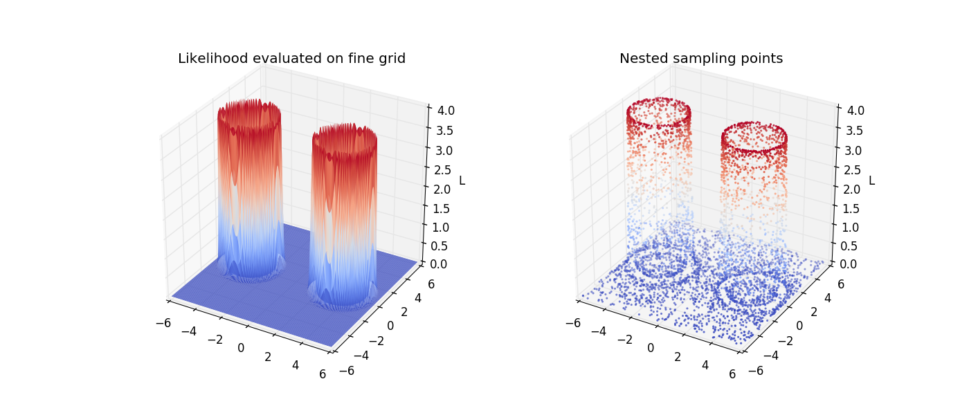
Gaussian Shells¶

Toy likelihood model for stress testing multiple-ellipsoid method.

The problem is:

\[\mathcal{L}(\theta) = \mathrm{circ}(\theta; c_1, r_1, w_1) + \mathrm{circ}(\theta; c_2, r_2, w_2)\]

where

\[\mathrm{circ}(\theta; c, r, w) = \frac{1}{\sqrt{2 \pi w^2}} \exp \left[ - \frac{(|\theta - c| - r)^2}{2 w^2} \right]\]

import math
import time
from collections import OrderedDict

import numpy as np
from numpy.random import RandomState
from matplotlib import pyplot as plt
from mpl_toolkits.mplot3d import Axes3D

import nestle

rstate = RandomState(0)

In the following block, we define the problem. We use r = 2 and w = 0.1, meaning that the gaussian is quite narrow compared to the size of the sphere.

r = 2.
w = 0.1

const = math.log(1. / math.sqrt(2. * math.pi * w**2))

def logcirc(theta, c):
    d = np.sqrt(np.sum((theta - c)**2, axis=-1))  # |theta - c|
    return const - (d - r)**2 / (2. * w**2)

def loglike(theta, c1, c2):
    return np.logaddexp(logcirc(theta, c1), logcirc(theta, c2))

def prior_transform(x):
    """Defines a flat prior between -6 and 6 in all dimensions."""
    return 12. * x - 6.

Visualize¶

It helps to visualize the surface in two dimensions. Here, we plot the likelihood evaluated on a fine grid and the sample points from nested sampling.

# likelihood surface in 2-d
xx, yy = np.meshgrid(np.linspace(-6., 6., 200),
                     np.linspace(-6., 6., 200))
c1 = np.array([-3.5, 0.])
c2 = np.array([3.5, 0.])
Z = np.exp(loglike(np.dstack((xx, yy)), c1, c2))

# nested sampling result
c1 = np.array([-3.5, 0.])
c2 = np.array([3.5, 0.])
f = lambda theta: loglike(theta, c1, c2)
res = nestle.sample(f, prior_transform, 2, method='multi', npoints=1000,
                    rstate=rstate)

fig = plt.figure(figsize=(14., 6.))
ax = fig.add_subplot(121, projection='3d')
ax.plot_surface(xx, yy, Z, rstride=1, cstride=1, linewidth=0, cmap='coolwarm')
ax.set_xlim(-6., 6.)
ax.set_ylim(-6., 6.)
ax.set_zlim(0., 4.)
ax.set_zlabel('L')
ax.set_title('Likelihood evaluated on fine grid')

ax = fig.add_subplot(122, projection='3d')
ax.scatter(res.samples[:,0], res.samples[:, 1], np.exp(res.logl),
           marker='.', c=np.exp(res.logl), linewidths=(0.,), cmap='coolwarm')
ax.set_xlim(-6., 6.)
ax.set_ylim(-6., 6.)
ax.set_zlim(0., 4.)
ax.set_zlabel('L')
ax.set_title('Nested sampling points');

Scaling with dimension¶

Here, we demonstrate how the algorithm scales with dimension and compare the total evidence to the analytic answer.

npoints = 1000

def run(ndim):
    """Convenience function for running in any dimension"""

    c1 = np.zeros(ndim)
    c1[0] = -3.5
    c2 = np.zeros(ndim)
    c2[0] = 3.5
    f = lambda theta: loglike(theta, c1, c2)

    return nestle.sample(f, prior_transform, ndim, method='multi',
                         npoints=npoints, rstate=rstate)

# Run over dimensions and save time for each run.
results = OrderedDict()
for ndim in [2, 5, 10, 20]:
    t0 = time.time()
    results[ndim] = run(ndim)
    results[ndim].time = time.time() - t0

analytic_logz = {2: -1.75,
                 5: -5.67,
                 10: -14.59,
                 20: -36.09}

print("D  analytic    logz  logzerr   nlike  eff(%)   time")
for ndim, res in results.items():
    eff = 100. * res.niter/(res.ncall - npoints)
    print("{:2d}   {:6.2f}  {:6.2f}     {:4.2f}  {:6d}   {:5.2f}  {:6.2f}"
          .format(ndim, analytic_logz[ndim], res.logz, res.logzerr,
                  res.ncall, eff, res.time))

Out:

D  analytic    logz  logzerr   nlike  eff(%)   time
  -1.75   -1.80     0.05   11912   37.55    1.64
  -5.67   -5.71     0.08   23413   35.74    5.11
 -14.59  -14.52     0.12   50193   34.19   10.97
 -36.09  -35.74     0.19  193214   19.78   40.58

Total running time of the script: ( 1 minutes 1.536 seconds)

Generated by Sphinx-Gallery